Stock Data & AR Models

The first step in this tutorial is to get access to WRDS (Wharton Research Data Services) which can be done here if you are a Kelley Student. You can also use Polygon or other stock data APIs

Assuming you are using WRDS, you'll need to get data this way:

!pip install wrds

import wrds
db = wrds.Connection()

Now, let's get data for a specific stock. WRDS allows you to pass in SQL to their API endpoints, so we'll do that. In this case, we'll be looking at GameStop stock.

gamestop_data = db.raw_sql("""
    SELECT
        dlycaldt,
        dlyret as daily_return,
        dlyprc as price,
        dlyvol as volume
    FROM crsp.dsf_v2
    WHERE ticker = 'GME'
    AND dlyret IS NOT NULL
    AND dlycaldt > '2000-01-01'
    ORDER BY dlycaldt
""")

import pandas as pd
df = pd.DataFrame(gamestop_data)

df['date'] = pd.to_datetime(df['dlycaldt'])
df.set_index('date', inplace=True)

Now, to make sure that there are no issues with our data by spot checking:

df

import matplotlib.pyplot as plt
import seaborn as sns
import numpy as np

# extracting the returns
returns = df['daily_return'].dropna()

plt.figure(figsize=(10, 6))
sns.histplot(data=returns, bins=50, kde=True, stat='density')
plt.title('Distribution of GameStop Daily Returns')
plt.xlabel('Daily Return')
plt.ylabel('Density')
plt.grid(True, alpha=0.3)

mean_return = returns.mean()
median_return = returns.median()
plt.axvline(mean_return, color='red', linestyle='--', label=f'Mean: {mean_return:.2%}')
plt.axvline(median_return, color='green', linestyle='--', label=f'Median: {median_return:.2%}')
plt.legend()

plt.gca().xaxis.set_major_formatter(plt.FuncFormatter(lambda x, _: f'{x:.0%}'))
plt.tight_layout()
plt.show()

print("Summary Statistics of Daily Returns:")
print(f"Mean: {returns.mean():.4%}")
print(f"Median: {returns.median():.4%}")
print(f"Standard Deviation: {returns.std():.4%}")
print(f"Min: {returns.min():.4%}")
print(f"Max: {returns.max():.4%}")
print(f"Skewness: {returns.skew():.4f}")
print(f"Kurtosis: {returns.kurtosis():.4f}")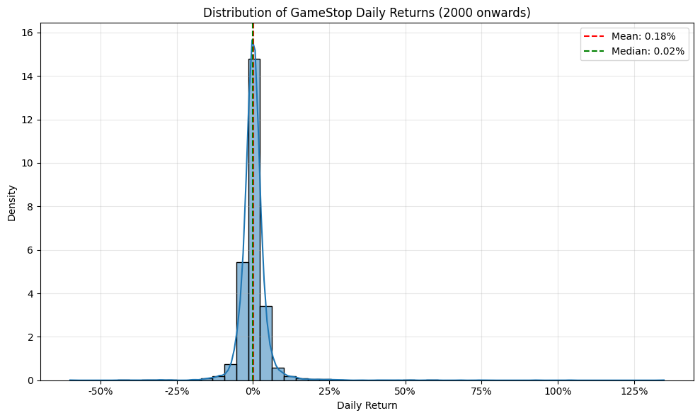

Summary Statistics of Daily Returns:
Mean: 0.1762%
Median: 0.0248%
Standard Deviation: 5.1278%
Min: -60.0000%
Max: 134.8358%
Skewness: 6.6967
Kurtosis: 149.1572

Is there a slight (actually massive) problem with this?

YES

We used raw return, which is NOT additive. We need to use log returns instead.

A 50% gain, and then a 33% loss are equivalent on the log scale as seen below:

log(150/100) + log(100/150) = 0

But not in raw form:

50% - 33% = 17%

Now, let's look at returns over time:

import matplotlib.pyplot as plt

plt.figure(figsize=(12, 6))
plt.plot(df.index, df['daily_return'], label='Daily Returns')
plt.title('GameStop (GME) Daily Returns')
plt.xlabel('Date')
plt.ylabel('Daily Return')
plt.grid(True, alpha=0.3)
plt.legend()

plt.xticks(rotation=45)

plt.tight_layout()

plt.show()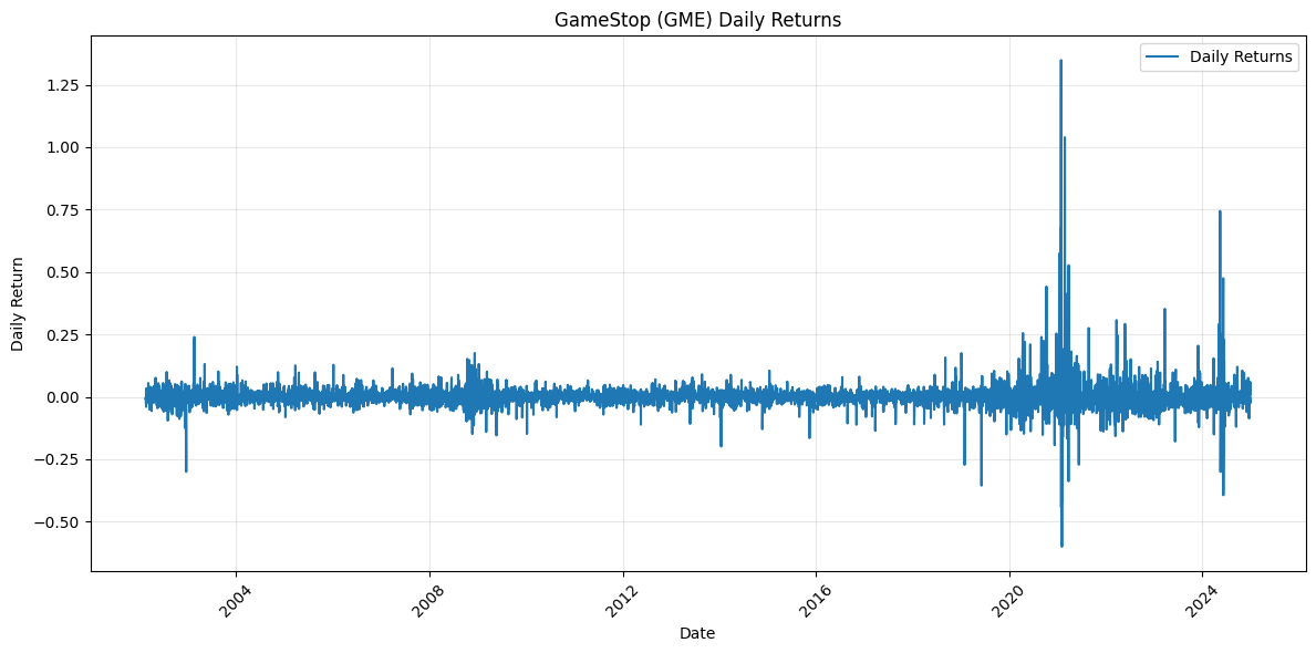

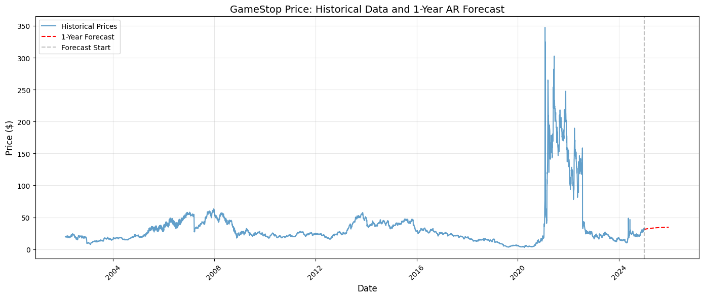
Notice where the volatility is? An option seller's biggest nightmare is to price an option for GameStop like it's 2016, and experience a massive uptick in volatility. This massive swing in volatility in one stock bankrupted several people in late 2021.